Data Science Workflow Tutorial

Step 1: Installation & Data Upload Notebook

Objective

• Set up a centralized environment for installing dependencies and loading static data
• Ensure reproducibility and easy recovery from kernel or system restarts
• Avoid redundant setup tasks across multiple notebooks

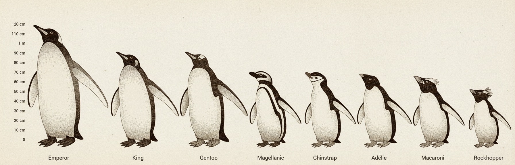
Exercise Instructions (Penguins dataset)

1. Create a new notebook and name it master_data.

2. Install the required libraries if not already installed (this step only needs to be run once per environment):

!pip install palmerpenguins
!pip install --upgrade setuptools

3. Import the necessary libraries for subsequent operations:

import pandas as pd
from palmerpenguins import load_penguins

4. Load the dataset:

penguins = load_penguins()

Alternatively, you can load the dataset directly from GitHub:

url = "https://raw.githubusercontent.com/allisonhorst/palmerpenguins/main/inst/extdata/penguins.csv"
penguins = pd.read_csv(url)

5. Publish the raw dataset as a DataCards variable, making it available to other notebooks:

dc.publish.variable(key="raw_penguins", value=penguins)

6. Preview the loaded data to confirm successful loading:

penguins.head()

Conceptual Takeaways

• Why centralize environment setup? Having a dedicated notebook for installation and data uploading ensures all team members use the same versions of dependencies and data, improving consistency and minimizing setup errors.

• Reproducibility: Storing data in shared variables allows the project to recover from kernel crashes or VM resets quickly without repeated data loading or reprocessing.

• Modularity: Separating environment setup and data ingestion from data preparation and modeling fosters a clean, maintainable workflow, reducing duplication of effort and enhancing collaboration.

• Scalability: This approach serves as the foundation for larger projects where multiple notebooks interact, helping manage computational resources more effectively.

Step 2: Main Data Handling Notebook

Objective

• Load, clean, and prepare the dataset for further analysis or modeling
• Keep environment setup and data logic modular
• Enable faster reruns after crashes or kernel restarts

Exercise Instructions

1. Create a new notebook and name it data_preparation

2. Load the raw dataset published in the previous step:

penguins = dc.consume.variable.raw_penguins()

3. Clean the data by dropping rows with missing values:

penguins = penguins.dropna()

4. Add a simple feature — a “BMI”-like metric:

penguins["bmi"] = penguins["body_mass_g"] / penguins["flipper_length_mm"]

5. Publish the cleaned dataset as a new DataCards variable:

dc.publish.variable(key="clean_penguins", value=penguins)

6. Optionally, display the cleaned data to verify the steps:

penguins

Conceptual Takeaways

• Modularity: Separating data cleaning and feature engineering into its own notebook keeps the workflow organized and logical, making it easier to maintain and debug.
• Efficiency: By publishing cleaned data as a separate variable, other notebooks can consume prepared data quickly without repeating time-consuming cleaning steps.
• Robustness: This structure supports smoother recovery from interruptions, since the environment setup and raw data loading happen independently from data transformation.
• Extensibility: The prepared data can be extended with additional features or transformations in this notebook before it feeds into modeling or visualization stages.

Step 3: Input/Filter Cards Notebook

Objective

• Separate filtering logic from data cleaning and final presentation
• Enable dynamic filter generation and flexible card layout
• Optimize memory usage by consolidating filter controls in a single notebook

Exercise Instructions

1. Create a new notebook and name it inputs.

2. Initialize filter variables with default values:

datacards.publish.variable("penguin_species", "Adelie")  # Default species
datacards.publish.variable("penguin_bill_length", 30)   
datacards.publish.variable("penguin_bill_depth", 15)
datacards.publish.variable("penguin_flipper_length", 190)  
datacards.publish.variable("penguin_sex", 0)  # 0 = Female, 1 = Male

3. Load the cleaned data from the previous notebook:

penguins = datacards.consume.variable.clean_penguins()

4. Generate options for the species combobox dynamically:

options = [str(s) for s in penguins["species"].unique()]
options

5. Publish a combobox card for species selection (make sure this code stays in one cell only):

datacards.publish.card(
    type='combobox',
    label='Species',
    options=options,
    variable_key='penguin_species',
    logic_view_size=(2,2),
    layout=[{"size": (3,2), "position": (0,0), "deck": "default-deck"}]    
)

6. Publish slider cards for filtering numeric inputs (use one publish.card per cell only):

dc.publish.card(
    type='floatSlider',
    label='Bill Length',
    unit='[mm]',
    min=30.0,
    max=60.0,
    step=0.5,
    variable_key='penguin_bill_length',
    logic_view_size=(3,1),
    layout=[{"size": (3,2), "position": (0,4), "deck": "default-deck"}]
)

dc.publish.card(
    type='floatSlider',
    label='Bill Depth',
    unit='[mm]',
    min=13.0,
    max=22.0,
    step=0.1,
    variable_key='penguin_bill_depth',
    logic_view_size=(3,1),
    layout=[{"size": (3,2), "position": (0,2), "deck": "default-deck"}]
)

dc.publish.card(
    type='floatSlider',
    label='Flipper Length',
    unit='[mm]',
    min=170.0,
    max=230.0,
    step=1.0,
    variable_key='penguin_flipper_length',
    logic_view_size=(3,1),
    layout=[{"size": (3,2), "position": (3,2), "deck": "default-deck"}]
)

7. Publish a toggle card for sex/gender selection:

dc.publish.card(
    type='toggle',
    label='Sex [♀/♂]',
    variable_key='penguin_sex',
    logic_view_size=(2,1),
    layout=[{"size": (3,2), "position": (3,0), "deck": "default-deck"}]
)

Conceptual Takeaways

• Separation of concerns: Keeping filtering controls distinct from data cleaning and modeling promotes a modular, maintainable architecture.
• Dynamic UI generation: Filter options can adapt automatically based on the dataset, which improves flexibility across projects.
• Memory optimization: Combining all filters in a single notebook reduces the number of active notebooks, saving RAM and improving performance.
• User interaction: Creating interactive filter cards provides a user-friendly way for stakeholders or analysts to explore and customize data views.

Step 4: Business Logic / Model Notebook

Objective

• Isolate core analytical and predictive computations apart from data preparation and visualization
• Enable iterative experimentation with different modeling approaches without repeating data loading or plotting
• Improve maintainability by allowing changes in business logic or model architecture without impacting other workflow components

Exercise Instructions

1. Create a new notebook and name it model.

2. Import required libraries:

import pandas as pd
import numpy as np
from sklearn.linear_model import LinearRegression
from sklearn.metrics import r2_score, mean_absolute_error

3. Load prepared data and user inputs published from previous notebooks:

penguins = datacards.consume.variable.clean_penguins()
penguin_species = datacards.consume.variable.penguin_species()
penguin_sex_raw = datacards.consume.variable.penguin_sex()
penguin_flipper_length = datacards.consume.variable.penguin_flipper_length()
penguin_bill_length = datacards.consume.variable.penguin_bill_length()
penguin_bill_depth = datacards.consume.variable.penguin_bill_depth()
 
# Convert boolean to integer: False=0 (Female), True=1 (Male)
penguin_sex = int(penguin_sex_raw)

4. Print user input for confirmation:

print(f'''The user identified a penguin of species {penguin_species} of sex {penguin_sex}.
The individual's bill is {penguin_bill_length} mm long,
depth {penguin_bill_depth} mm, and flipper length is {penguin_flipper_length} mm.
''')

5. Inspect the loaded data (optional):

penguins

6. Encode categorical variables for modeling:

penguins_encoded = pd.get_dummies(penguins, columns=['species', 'sex'], drop_first=False)
feature_cols = ['bill_length_mm', 'bill_depth_mm', 'flipper_length_mm'] + \
               [col for col in penguins_encoded.columns if col.startswith(('species_', 'sex_'))]
 
X = penguins_encoded[feature_cols]
y = penguins_encoded['bmi']  # Target variable

7. Train linear regression model:

model = LinearRegression()
model.fit(X, y)

8. Evaluate model performance:

y_pred = model.predict(X)
r2 = r2_score(y, y_pred)
mae = mean_absolute_error(y, y_pred)

9. Print regression formula and model metrics:

print("=" * 60)
print("BMI REGRESSION FORMULA")
print("=" * 60)
print(f"\nBMI = {model.intercept_:.3f}")
for name, coef in zip(feature_cols, model.coef_):
    print(f"      {coef:+.3f} * {name}")
print("\n" + "=" * 60)
print("MODEL PERFORMANCE")
print("=" * 60)
print(f"R² Score: {r2:.4f}")
print(f"MAE:      {mae:.4f}")

10. Create a user input DataFrame matching model features and make a prediction:

user_data = pd.DataFrame({
    'bill_length_mm': [penguin_bill_length],
    'bill_depth_mm': [penguin_bill_depth],
    'flipper_length_mm': [penguin_flipper_length],
    'species': [penguin_species],
    'sex': ['Female' if penguin_sex == 0 else 'Male']
})
 
user_encoded = pd.get_dummies(user_data, columns=['species', 'sex'])
 
for col in feature_cols:
    if col not in user_encoded.columns:
        user_encoded[col] = 0
 
user_encoded = user_encoded[feature_cols]
 
predicted_bmi = model.predict(user_encoded)[0]

11. Output user prediction:

print(f"\nInput values:")
print(f"  Species:        {penguin_species}")
print(f"  Sex:            {'Female' if penguin_sex == 0 else 'Male'}")
print(f"  Bill length:    {penguin_bill_length} mm")
print(f"  Bill depth:     {penguin_bill_depth} mm")
print(f"  Flipper length: {penguin_flipper_length} mm")
print(f"\n➤ Predicted BMI: {predicted_bmi:.3f}")

12. Publish predicted BMI as a DataCards variable:

dc.publish.variable("predicted_bmi", predicted_bmi)

13. Create and publish a compact regression formula string showing significant coefficients:

significant_coefs = [(name, coef) for name, coef in zip(feature_cols, model.coef_) if abs(coef) > 0.001]
formula_string = f"BMI = {model.intercept_:.3f}"
for name, coef in significant_coefs[:5]:  # top 5 coefficients
    formula_string += f" {coef:+.3f}*{name}"
dc.publish.variable("bmi_formula", formula_string)

14. Publish a number card displaying predicted BMI:

dc.publish.card(
    type='number',
    value=predicted_bmi,
    label='Predicted BMI',
    unit='kg/m²',
    decimals=2,
    logic_view_size=(2, 1),
    layout=[{"size": (3,2), "position": (3,4), "deck": "default-deck"}]
)

Conceptual Takeaways

• Separation of concerns: Complex modeling logic is isolated from data preparation and visualization to enhance clarity and maintainability.

• Iterative modeling: This setup facilitates trying out different models or analytical approaches without redoing upstream steps.

• Model transparency: Printing out regression formulas and performance metrics helps understand model behavior and fit quality.

• User-driven predictions: Encoding user inputs consistently and feeding them into the model provides personalized predictive insights.

• Publishing results: Sharing predictions and formulas as variables and cards supports smooth integration into dashboards or further analysis steps.

Step 5: Visualization Notebook / Result Display

Objective

• Communicate findings effectively by turning complex insights into clear, intuitive visuals
• Support decision-making with business-ready presentations suitable for non-technical stakeholders
• Separate presentation from computation to enable independent updating of visuals without rerunning heavy data processing

Exercise Instructions

1. Create a new notebook and name it visualization.

2. Import required libraries and enable dark mode styling:

import matplotlib.pyplot as plt
import numpy as np
import pandas as pd
 
plt.style.use('datacards-dark-mode')

3. Consume required variables from previous notebooks:

penguins = datacards.consume.variable.clean_penguins()
selected_species = datacards.consume.variable.penguin_species()
predicted_bmi = datacards.consume.variable.predicted_bmi()
selected_sex = datacards.consume.variable.penguin_sex()
 
print(f"Creating BMI visualization for {selected_species} penguins")
print(f"Predicted BMI: {predicted_bmi:.2f}")
print(f"Selected sex: {'Male' if selected_sex else 'Female'}")

4. Filter data for the selected species:

species_data = penguins[penguins['species'] == selected_species].copy()

5. Separate data by sex for visual differentiation:

female_data = species_data[species_data['sex'] == 'female']['bmi']
male_data = species_data[species_data['sex'] == 'male']['bmi']

6. Create a figure of adequate size for DataCards layout:

fig, ax = plt.subplots(figsize=datacards.utilities.plotting.plot_area(rows=4, columns=6))

7. Plot histograms for female and male BMI distributions:

bins = np.linspace(species_data['bmi'].min(), species_data['bmi'].max(), 20)
 
ax.hist(female_data, bins=bins, alpha=0.7, label='Female', color='#ff6b9d', edgecolor='white', linewidth=0.5)
ax.hist(male_data, bins=bins, alpha=0.7, label='Male', color='#4ecdc4', edgecolor='white', linewidth=0.5)

8. Add a vertical line indicating the predicted BMI:

ax.axvline(predicted_bmi, color='#ffd93d', linewidth=1, linestyle='--', label=f'Prediction: {predicted_bmi:.1f}')

9. Customize axes labels and grid:

ax.set_xlabel('BMI (kg/m²)', fontsize=12)
ax.set_ylabel('Frequency', fontsize=12)
# **Note:** Avoid titles and legends in DataCards dashboards per best practice
ax.grid(True, alpha=0.3)

10. Adjust layout and publish the visualization as a DataCards matplotlib card:

plt.tight_layout()
 
datacards.publish.card(
    type='matplotlib',
    fig=fig,
    label=f'BMI Distribution - {selected_species}',
    logic_view_size=(6, 4),
    layout=[{"size": (20, 1), "position": (0, 9), "deck": "default-deck"}]
)

Conceptual Takeaways

• Effective communication: Visualizing distributions helps stakeholders quickly grasp the data and understand predictions in context.

• Separation of concerns: This notebook focuses solely on presentation; analytical computations are kept separate for modularity and performance.

• Interactivity readiness: Published cards can be integrated into dashboards, enabling dynamic interactions with filtered or predicted data.

• Design principles: Following DataCards best practices (e.g., avoiding titles/legends inside cards) ensures clean, professional dashboards.